New mill

A new concept of calculating the required machining power when milling.

Courtesy of Walter

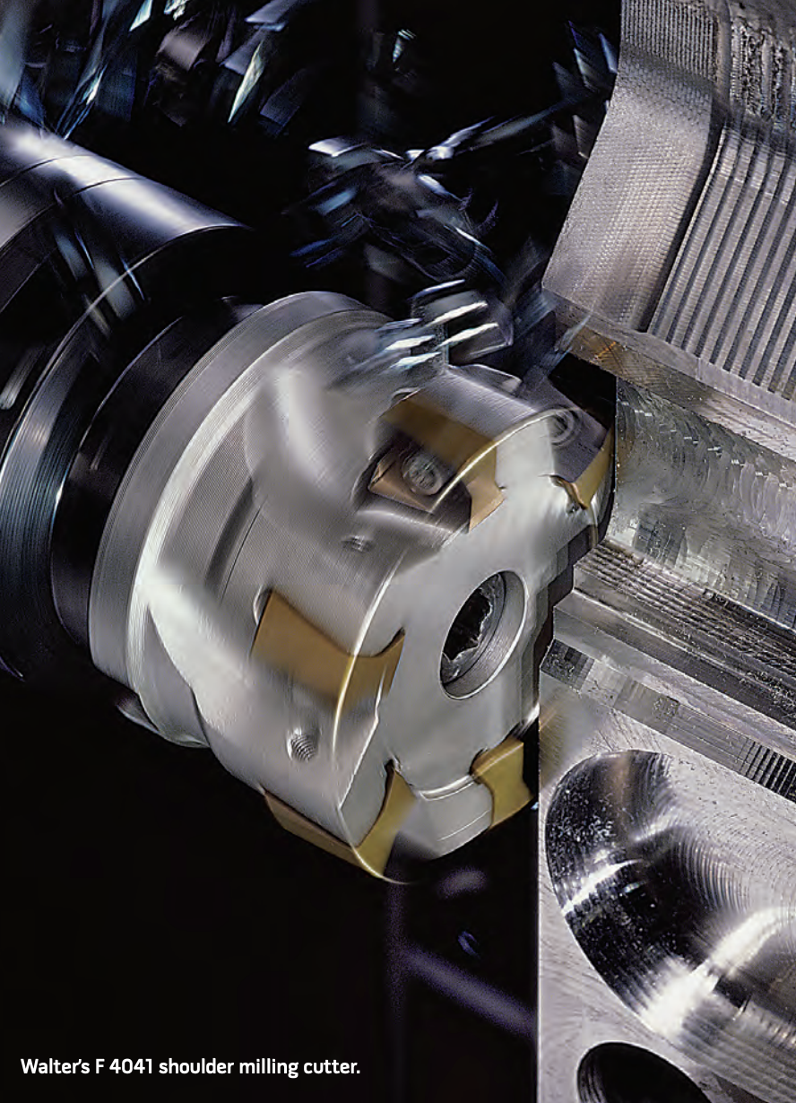
Walter’s F 4041 shoulder milling cutter.

The conventional method of calculating required machining power (Pr) is based on the metal-removal rate, measured in in.3/min. (cm3/min.), and the average unit power requirements (Pm), measured in hp/in.3/min. (kW/cm3/min.). The formula for calculating required machining power is Pr = mrr × Pm. The method has been used since the 1960s and has flaws.

For example, there is no data in the “Hardness” column between 200 HB and 35 HRC (Table 1). Because 35 HRC equals 327 HB, the gap is 127 HB. Unfortunately, the unit power data isn’t provided at the hardness from 200 to 327 HB. 

In addition, Table 1 indicates the hardness number is “80 HRB” for “copper,” which is confusing. Is it a specific grade of copper? Does “copper” mean more than one grade? It’s hard to tell. There are two copper grades: C10100 and 10200 (99.99 percent Cu), whose hardness after the H80 temper is 80 HRB. The table indicates the minimal hardness of copper alloys is 10 HRB (temper H00). However, the hardness of wrought copper alloys depends on the alloying elements and their amounts and therefore varies from 25 to 100 HRB, meaning there are no wrought copper alloys with a hardness of 10 HRB.

The simplicity of this conventional method makes it popular for calculating machining power, but it is not accurate. A unit power requirement (Pm) is not really a constant value. It depends on many factors, including workpiece hardness, milling cutter geometry and the cutting parameters. As the table shows, the majority of work materials are characterized by a broad hardness range with a single average Pm value. For example, the Pm is 1.5 for the hardness range from 150 to 450 HB, which is too big of a range. It means the average unit of power requirement is not an accurate quantity. Therefore, the old method should not be used for calculating required machining power.

You can calculate the MRR with this Online Calculator

Table 1. Average Unit Power Requirements (P_m) for Milling

Material	Hardness	Unit Power Requirements for HSS and Carbide Tools (Feed 0.005 to 0.012 ipt)
		Sharp Tool	Dull Tool
Steels, wrought and cast: Plain carbon, alloy steels and tool steels	85 to 200 HB	1.1	1.4
	35 to 40 HRC	1.5	1.9
	40 to 50 HRC	1.8	2.2
	50 to 55 HRC	2.1	2.6
	55 to 58 HRC	2.6	3.2
Cast irons: Gray, ductile and malleable	110 to 190 HB	0.6	0.8
	190 to 320 HB	1.1	1.4
Stainless steels, wrought and cast ferritic, austenitic and martensitic	135 to 275 HB	1.4	1.7
	30 to 45 HRC	1.5	1.9
Precipitation hardening stainless steels	150 to 450 HB	1.5	1.9
Titanium alloys	250 to 375 HB	1.1	1.4
High-temperature alloys: Nickel, cobalt and iron base	200 to 360 HB	2.0	2.5
	180 to 320 HB	1.6	2.0
Refractory alloys: Tungsten, molybdenum, niobium and tantalum	321 HB	2.9	3.6
	229 HB	1.6	2.0
	217 HB	1.5	1.9
	210 HB	2.0	2.5
Nickel alloys	80 to 360 HB	1.9	2.4
Aluminum alloys	30 to 150 HB (500-kg load)	0.32	0.4
Magnesium alloys	40 to 90 HB (500-kg load)	0.16	0.2
Copper	80 HRB	1.0	1.2
Copper alloys	10 to 80 HRB	0.64	0.8
	80 to 100 HRB	1.0	1.2

The table is adapted from the Machining Data Handbook, Third Edition, Vol. 2, pg. 17-10, published in 1980 by Metcut Research Associates Inc., Cincinnati. (The First Edition was published in 1966.) “Titanium” and “Columbium” (as they appear in the original table, column Material) were renamed “Titanium alloys” and “Niobium,” respectively. Hardness abbreviations (column Hardness) were changed to present them as they are currently used: HB (Brinell hardness) replaced “Bhm”; HRC (Rockwell hardness, C scale) replaced “RC,” and HRB (Rockwell hardness, B scale) replaced “RB.”

New Calculation Method 

To increase accuracy when calculating machining power, the author developed a new method based on the definition of power (P) as a product of the cutting force (F) and the cutting speed (VC):

P = F (lbs.) × VC (sfm) ÷ 33,000 (hp) 

or P = F (N) × VC (m/min.) ÷ 60,000 (kW)

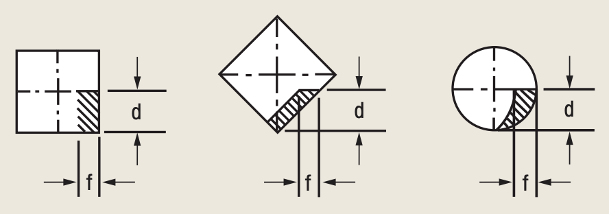
Figure 1. Cross sections of uncut chips produced by square and round inserts.

Because cutting speed is one of the selectable machining parameters, only the cutting force should be calculated to obtain the required machining power. 

Equations for calculating the cutting force when milling can be found in various technical papers and books. However, these equations include complex trigonometric functions, integrals and matrices, and some of the formulas are second-order differential equations. Such complex equations are not appropriate in practical engineering calculations because only mathematicians proficient in calculus can execute them. Therefore, simple algebraic equations are needed to perform similar calculations within a practical range of accuracy, which is ±20 percent or better.

Simplified equations should only contain parameters that significantly impact the cutting force. These parameters are included in the new method. 

An analytical study of metalcutting principles and analyses of numerous milling tests the author conducted resulted in a new concept for calculating the cutting force. The new concept is based on the relationships between the following parameters:

• Ultimate tensile strength of a workpiece vs. its hardness, 

• Cross-sectional area of the uncut chip vs. axial DOC and feed per tooth,

• Number of teeth in the cut vs. number of teeth in a cutter and radial WOC,

• Engagement factor vs. radial WOC, cutter diameter and workpiece material, and 

• Tool wear factor vs. axial DOC and feed per tooth.

The cutting force (F) formula is based on those relationships:

F = σ × A × ZC × CE × CW (1), where:

σ is the workpiece’s ultimate tensile strength in psi or MPa,

A is the chip’s cross-sectional area in in.2 or mm2, 

ZC is the number of teeth (inserts) in the cut,

CE is the engagement factor, and

CW is the cutting tool wear factor.

Ultimate Tensile Strength

The author developed numerous statistical and linear regression formulas for calculating the ultimate tensile strength of carbon, alloy, stainless and tool steels based on their Brinell hardness numbers. 

Because of space limitations, only linear regression formulas for calculating ultimate tensile strength (σ) vs. Brinell hardness number (HB) are provided for AISI 1050 carbon steel and AISI 4140 alloy steels.

AISI 1050 grade, 235 HB: 

σ = 501 × HB – 568 (2)

σ = 501 × 235 – 568 = 117,167 psi

(The actual ultimate tensile strength is 117,200 psi)

Formula (2) provides 98 to 100 percent accuracy in calculating ultimate tensile strength. Its application is limited to the Brinell hardness range from 160 to 270 HB.

AISI 4140 grade, 229 HB: 

σ = 506 × HB – 3,456 (3)

σ = 506 × 229 – 3,456 = 112,418 psi

(The actual ultimate tensile strength is 112,000 psi)

Formula (3) provides 97.1 to 99.9 percent accuracy in calculating ultimate tensile strength. Its application is limited to the Brinell hardness range from 195 to 580 HB.

Cross-Sectional Area 

The shape of an uncut chip’s cross section depends on insert geometry and the milling cutter’s lead angle. Round inserts produce chips in the shape of a partial crescent. Inserts of all other shapes with straight cutting edges produce chips with either a rectangular cross section for milling cutters with a 0° lead angle or a parallelogram cross section for milling cutters with lead angles greater than 0°. Cross sections of the chips produced by square inserts (0° and 45° lead angles) and a round insert are shown in Figure 1. 

The cross-sectional area of the chip (A) is a product of the axial DOC (d) and feed per tooth (f):

A = d × f (4) 

Formula (4) is easily understood when applied to rectangular and parallelogram cross-sectional areas, but it is not so obvious when the formula is applied to a cross-sectional area of a chip produced by a round insert. Then, the cross-sectional area is either a half-crescent when the axial DOC equals the insert’s radius, or smaller than a half-crescent when the axial DOC is less than the insert’s radius. The applicability of formula (4) for crescent-like areas has been proven by integral calculus and algebraic-trigonometric calculations.

Number of Engaged Inserts

A typical facemilling cutter has three or more teeth (inserts), but only a few of them are simultaneously engaged with the workpiece. The number of inserts in a cut (ZC) depends on the number of inserts in a cutter (Z) and the engagement angle (α). This relationship is expressed by the formula:

ZC = Z × α ÷ 360 (5)

The engagement angle depends on the radial WOC (W) and cutter diameter (D). This angle is shown in Figures 2 and 3, which illustrate the two most typical positions of a milling cutter when engaged with a workpiece.

Table 2. Number of inserts in the cut vs. W:D ratio.

W:D	0.85	0.80	0.75	0.70	0.60	0.45	0.35	0.20	0.15
ZC	0.37 Z	0.35 Z	0.33 Z	0.32 Z	0.28 Z	0.23 Z	0.20 Z	0.15 Z	0.13 Z

Table 3. Engagement factors vs. W:D ratio.

Workpiece material	W:D ≤ 0.5	0.5 < W:D ≤ 0.7	0.7 < W:D = 1
Carbon and alloy steels	1.0	1.3	1.5
Stainless and tool steels	1.6	1.8	2.2

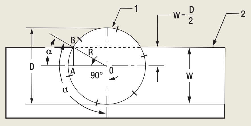
Figure 2. The centerline of the cutter (1) is located on the workpiece (2).

Figure 2 shows a cutter’s centerline on a workpiece, with the engagement angle greater than 90°. The maximum engagement angle possible is 180°, occurring when the radial WOC equals the cutter diameter. In such a case, half of the inserts are engaged with the workpiece material. If the radial WOC equals the cutter radius, only 25 percent of the inserts are engaged with the workpiece. The number of inserts in the cut can be found for any WOC using the following formulas.

As seen in Figure 2, the engagement angle (α) equals 90° plus α1, where α1 is the angle between the cutter diameter and the cutter radius R drawn to the peripheral point B at the entry or exit.

From the right-angle triangle OAB: 

sin α1 = AB ÷ OB = (W – R) ÷ R = (W – D ÷ 2) ÷ (D ÷ 2) = (2W – D) ÷ D, 

α1 = arc sin [(2W – D) ÷ D] and the engagement angle is:

α = 90° + arc sin [(2W – D) ÷ D] (6)

Substitution of α from formula (6) into formula (5) gives:

ZC = Z × (90° + arc sin [(2W – D) ÷ D)] ÷ 360 (7)

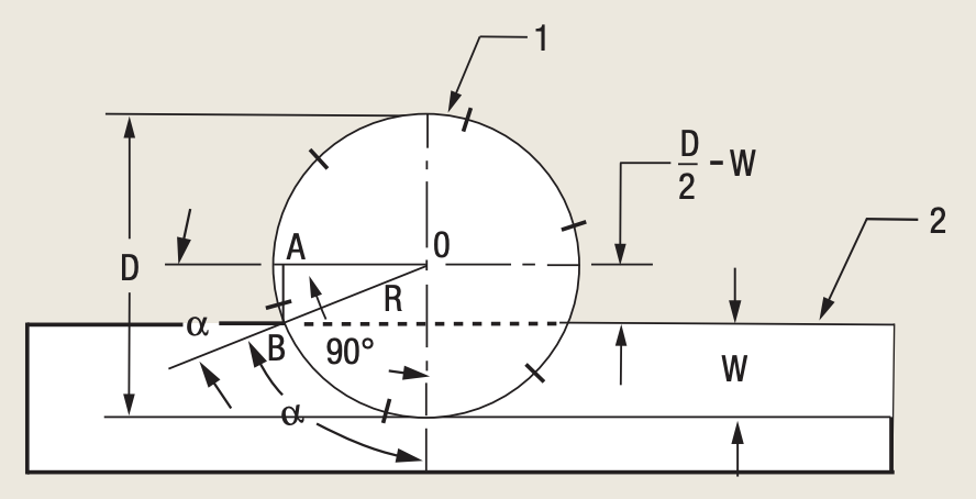
Figure 3. The centerline of the cutter (1) is not located on the workpiece (2).

Figure 3 shows a cutter’s centerline that is not located on a workpiece, so the radial WOC is less than the cutter radius. Therefore, the engagement angle is less than 90°.

As seen in Figure 3, the engagement angle (α) equals 90° minus α1, where α1 is the angle between the cutter’s centerline and the cutter radius R drawn to the peripheral point B at the entry or exit.

From the right-angle triangle OAB: 

sin α1 = AB ÷ OB = (R – W) ÷ R = (D ÷ 2 – W) ÷ (D ÷ 2) = (D – 2W) ÷ D,

α1 = arc sin [(D – 2W) ÷ D] and the engagement angle is:

α = 90° – arc sin [(D – 2W) ÷ D] (8)

Substitution of α from formula (8) into formula (5) gives:

ZC = Z × (90° – arc sin [(D – 2W) ÷ D)] ÷ 360 (9)

If you don’t have a calculator with trigonometric functions, Table 2 helps to estimate the number of inserts in the cut based on the ratio of the radial WOC (W) to cutter diameter (D).

Engagement Factor

The engagement factor (CE) is a dimensionless quantity that depends on the ratio of the radial WOC (W) to the cutter diameter (D) and the type of workpiece.

Milling is more effective when it produces sufficiently thick and uniform chips. The W:D ratio determines chip thickness uniformity. When the radial WOC equals cutter diameter (W ÷ D = 1), the chip being formed starts at zero thickness at the point of entry and then thickness increases to its maximum at the cutter’s centerline and thins to zero at the exit point. This type of cut produces a nonuniform chip, which generates maximum friction at the cutting edge and increases cutting resistance.

Effective facemilling is obtained when W:D ≈ 2:3 or W ≈ 0.7 D. This type of cut produces uniform and sufficiently thick chips, which generates minimal friction at the cutting edge and decreases cutting resistance. Engagement factors are given in Table 3.

Wear Factor

The cutting tool wear factor (CW) is a dimensionless quantity that depends on the cutting parameters. When milling with new or freshly indexed inserts until the flank wear does not exceed about 0.004 " to 0.005 ", the cutting tool wear factor is 1.0. When milling until the inserts are indexed or replaced (the tool life reached 100 percent), the following cutting tool wear factors are recommended, according to the milling category:

• Light facemilling, CW = 1.1

• Medium facemilling, CW = 1.2

• Heavy-duty facemilling, CW = 1.3

Table 4. Milling categories and tool wear factors.

Milling category	Axial DOC, in.	Feed per tooth, in.	Cross-sectional area of the chip, in.2	Cutting tool wear factor, CW
Light	0.020 to 0.100	0.003 to 0.006	0.00006 to 0.0006	1.1
Medium	0.100 to 0.200	0.006 to 0.010	0.0006 to 0.002	1.2
Heavy duty	0.200 to 0.400	0.010 to 0.020	0.002 to 0.008	1.3

Unfortunately, the author could not find any information that defines these milling categories and prepared a questionnaire asking for machining data that best describes the milling categories by a certain range of the axial DOC and feed per tooth. The questionnaire was sent to more than 100 people with practical knowledge and experience in milling. Statistical treatment of their responses is found in Table 4.

Required Machining Power 

The following machining power calculations are performed using the conventional method and the new method to compare them. 

• The work material is annealed AISI 4140 alloy steel with a Brinell hardness of 180 HB. According to Walter USA LLC’s material classification, 4140 alloy steel belongs to group 6.

• The cutting tool is Walter’s shoulder milling cutter F 4041.

Description, 4041.UB.102.Z08.13 

Diameter, DC = 4.0 "

Number of inserts, Z = 8

Approach angle, κ = 90° (similar to a 0° lead angle)

Coated grade, WKP 25

• The machining data for roughing was adopted from Walter’s general catalog from 2007.

Starting value for cutting speed, VC = 850 sfm

Feed rate per tooth, fZ0 = 0.006 "

DOC, ap = 0.400 "

WOC, ae = 2.6 "

ae ÷ DC = 0.65

As previously noted, the formula for the conventional method is Pr = mrr × Pm. 

• The mrr and cutter rpm:

mrr = ap × ae × fZ0 × Z × n, where n = 12 × VC ÷ (π × DC) 

n = 12 × 850 ÷ (π × 4) = 812 rpm

mrr = 0.4 × 2.6 × 0.006 × 8 × 812 = 40.5 in.3/min.

• Required machining power, sharp tool (Pm = 1.1, from Table 1):

Pr = mrr × Pm = 40.5 × 1.1 = 44.5 hp

• Required machining power, dull tool (Pm = 1.4, from Table 1):

Pr = mrr × Pm = 40.5 × 1.4 = 56.7 hp

The following information is used for the new method.

• Ultimate tensile strength (σ) of AISI 4140 alloy steel, 180 HB; formula (3):

σ = 506 × HB – 3,456 = 506 × 180 – 3,456 ≈ 87,600 psi (after rounding off)

• Cross-sectional area of the chip, formula (4):

A = ap × fZ0 = 0.4 × 0.006 = 0.0024 sq. in.

• Number of inserts engaged with the workpiece, formula (7):

ZC = 8 × (90° + arc sin [(2 × 2.6 – 4) ÷ 4)] ÷ 360 = 8 × (90° + 17.46°) ÷ 360 = 2.4

• Engagement factor (CE), Table 3:

For ae ÷ DC = 0.65 and 4140 alloy steel, CE = 1.3

• Tool wear factor (CW), Table 4:

For 0.0024-sq.-in. cross-sectional area of the chip, CW = 1.3

• Cutting force, sharp tool:

F = σ × A × ZC × CE = 87,600 × 0.0024 × 2.4 × 1.3 = 656 lbs.

• Cutting force, dull tool:

F = σ × A × ZC × CE × CW = 87,600 × 0.0024 × 2.4 × 1.3 × 1.3 = 853 lbs.

• Required machining power, sharp tool:

Pr = F × VC ÷ 33,000 = 656 × 850 ÷ 33,000 = 16.9 hp

• Machining power at the motor, sharp tool:

PM = Pr ÷ η, where η is a machine efficiency factor (η = 0.8 to 0.95) 

Assuming η = 0.8 (the same value as used in the conventional method):

PM = 16.9 ÷ 0.8 = 21.1 hp

• Required machining power, dull tool: Pr = 853 × 850 ÷ 33,000 = 22.0 hp

• Machining power at the motor, dull tool: PM = 22 ÷ 0.8 = 27.5 hp

The machining power values calculated using the new method:

Milling with sharp tool, PM = 21.1 hp

Milling with dull tool, PM = 27.5 hp

The machining power values calculated using the conventional method:

Milling with sharp tool, PM = 44.5 hp

Milling with dull tool, PM = 56.7 hp

This shows that the machining power calculated by the conventional method is more than twice the power calculated by the new method!

New Method Machining Power Calculator for Milling

Ultimate Tensile Strength (σ) in psi:
Cross-sectional Area (A) of Chip in sq. in.:
Number of Inserts in Cut (ZC):
Engagement Factor (CE):
Tool Wear Factor (CW):
Cutting Speed (VC) in sfm:
Machine Efficiency Factor (η):
Calculate Machining Power

Results:

Formula for Cutting Force (F): F = σ × A × ZC × CE × CW

Formula for Required Machining Power (Pr): Pr = F × VC ÷ 33,000

Formula for Machining Power at Motor (PM): PM = Pr ÷ η, where η is the machine efficiency factor

Cutting Tool Engineering and the author invite readers to participate in a discussion regarding these two methods of calculating the required machining power when milling. Please share your experiences and opinions. CTE

About the Author: Edmund Isakov, Ph.D., is a consultant, writer and frequent contributor to Cutting Tool Engineering. He is the author of the books “Mechanical Properties of Work Materials” (Modern Machine Shop Publications, 2000), “Engineering Formulas for Metalcutting” (Industrial Press, 2004) and “Cutting Data for Turning of Steel” (Industrial Press, 2009) and the software “Advanced Metalcutting Calculators” (Industrial Press, 2005). He can be e-mailed at edmundisakov@bellsouth.net or reached at (561) 369-4063.